# load packages
library(AER)
library(stargazer)
library(ggplot2)
library(GGally) # scatterplots via GGpairs
library(lmtest) # BP test, coeftest
library(car) # vif test for MC,

# Load and prepare data
?CPS1985
data("CPS1985")
rownames(CPS1985) <- index(CPS1985)Outliers
Intro to Stats
Regression
Diagnostics
This brief guide is supposed to explain the interpretation of dfBetas, both standardised and non-standardised. I load data and packages above. Note that I assigned the index of our data as the rownames. Taking care of this at the beginning of your script helps improve the interpretability of your plots to identify outliers (sometimes the rownames might be random numbers, this way you make sure that the rownames run from 1 to the number of observations). After preparing the data in this way (and dropping possible outliers), we fit our model of interest:
m3 <- lm(wage ~ education + experience*gender, data = CPS1985) # Model with interaction.
summary(m3)
Call:
lm(formula = wage ~ education + experience * gender, data = CPS1985)

Residuals:
    Min      1Q  Median      3Q     Max
-10.262  -2.518  -0.659   1.842  36.863

Coefficients:
                        Estimate Std. Error t value Pr(>|t|)
(Intercept)             -5.03445    1.21323  -4.150 3.88e-05 ***
education                0.94859    0.07833  12.110  < 2e-16 ***
experience               0.15824    0.02240   7.065 5.08e-12 ***
genderfemale            -0.67455    0.67726  -0.996  0.31971
experience:genderfemale -0.09277    0.03107  -2.986  0.00296 **
---
Signif. codes:  0 '***' 0.001 '**' 0.01 '*' 0.05 '.' 0.1 ' ' 1

Residual standard error: 4.421 on 529 degrees of freedom
Multiple R-squared:  0.2655,    Adjusted R-squared:   0.26
F-statistic: 47.81 on 4 and 529 DF,  p-value: < 2.2e-16
You know these estimates from the lab, so I am going to check for outliers right away, using avPlots():
avPlots(m3)
Remember that these plots show the relationship of each indpendent with your dependent variable, controlling for all other variables. This way, we can see what the correlation of the variables in the model looks like. Simple scatterplots do not take into account that some of the variation is explained by other variables.
We can see that observation #171 is somewhat of an outlier, always showing strong discrepancy (deviation from the predicted values). It also shows some leverage, as it deviates somewhat from the average value for gender, controlling for all other variables. It is quite possible that it would affect our estimates hence. We can check if that is the case using dfBetas:
dfbetasPlots(m3, id.n=5, labels=rownames(CPS1985))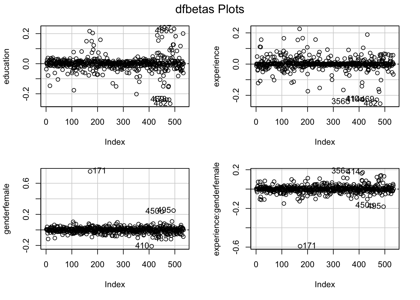
Remember that dfbetasPlots() shows how strongly a single observation affects your model estimates. It does so by estimating the model, dropping each observation once. Then, it calculates the standard deviation and indicates by how many standard deviations the effect would change. While the estimates for education and experience seem rather unaffected by single observations, observation #171 deviates quite a bit from the overall trend. Note that this is not a lot in terms of standard deviations (around 0.7 sd for gender, -0.6 for the interaction coefficient), so we could conclude that the estimate is not strongly effected and that we do not have outliers. But since we are cautious sticklers, we will estimate how much our model is affected. We can check this (to be sure) by using dfbetaPlots(), which shows the non-standardised deviation in the effect (we’re focusing on the gender variable here):
dfbetaPlots(m3, ~gender, id.n=5, labels=rownames(CPS1985))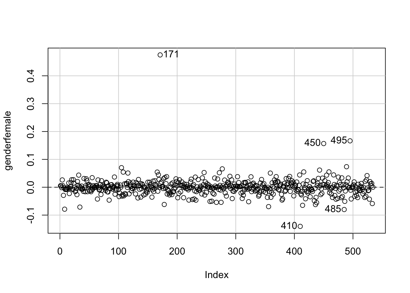
The scale has changed, as it now shows the absolute effect of the outlier on gender. Observation #171 biases the estimate upwards by something between 0.4 and 0.5. Given that the estimate from our model above was -0.67, with a standard error of 0.68, this is a substantial effect for a single observation, despite the fact that it is \(<1\) standard deviation in the dfbetasPlot(). So - to be sure - let’s estimate a model without the outlier:
m3_robust <- lm(wage ~ education + experience*gender, data = CPS1985[-171,]) # Model without outlier
stargazer(m3, m3_robust, type = "text", column.labels = c("Full data", "No Outliers"))
=======================================================================
                                      Dependent variable:
                        -----------------------------------------------
                                             wage
                               Full data              No Outliers
                                  (1)                     (2)
-----------------------------------------------------------------------
education                      0.949***                0.951***
                                (0.078)                 (0.073)

experience                     0.158***                0.158***
                                (0.022)                 (0.021)

genderfemale                    -0.675                  -1.150*
                                (0.677)                 (0.633)

experience:genderfemale        -0.093***               -0.076***
                                (0.031)                 (0.029)

Constant                       -5.034***               -5.074***
                                (1.213)                 (1.131)

-----------------------------------------------------------------------
Observations                      534                     533
R2                               0.266                   0.301
Adjusted R2                      0.260                   0.295
Residual Std. Error        4.421 (df = 529)        4.120 (df = 528)
F Statistic             47.813*** (df = 4; 529) 56.740*** (df = 4; 528)
=======================================================================
Note:                                       *p<0.1; **p<0.05; ***p<0.01
Note that we can only drop the outlier this simple (CPS1985[-171,]) since we assigned the index as rownames with rownames(CPS1985) <- index(CPS1985) earlier. As you can see, the estimate for gender changed from \(-0.675\) to \(-1.150\) - a change of \(-0.475\)! This is the dfbeta (non-standardised) for observation #171 and also what is displayed in dfbetaPlots() above - #171 biased the estimate upward by \(0.475\) (see below). Also note that - in line with our expectation based on the dfbetasPlots() earlier - the estimate for the interaction increased (decreased in size).
as.data.frame(dfbeta(m3))[171, "genderfemale"][1] 0.4749832Note that this last bit is only included to explain the concept of dfbeta to you - you are not expected to show this in your FDA! The ‘secure’ way would be to include the model with outliers in the appendix and to report the slight changes with an overall similar interpretation of the model.